Cell scatter plot — clustering & gating

Extensions → SP Classify → Scatter Plots and Clustering... opens a scatter plot for unsupervised clustering. Cells are clustered on their marker measurements with k-means or Leiden (§11.6) and drawn on a 2D PCA or UMAP plot. You can then name the clusters as QuPath classes. This does not use or change the trained classifier or its training labels.

When the window opens, pick the measurements to use in the Select Measurements for Scatter Plot dialog. The window then loads the open image's cells (up to the Sample: cap, default 50,000) and shows "… cell(s) loaded — click “Recompute” to cluster." Click Recompute to cluster and draw the plot.

Clustering uses the normalisation set in Clustering Normalisation (§4.2). The classifier always uses raw values. Each marker is then z-scored over the cells being clustered. If you change the normalisation while a plot exists, reopening the plot from the menu asks whether to build a new plot with the new normalisation (the current clusters are discarded) or keep the existing plot. New clustering session always uses the current normalisation.

11.1 Controls

Top row - Embedding — PCA (fast) or UMAP (slower; often separates overlapping populations better). The embedding only positions the points on the plot. Clustering always uses the marker values, not the 2D coordinates. - Full UMAP (UMAP only) — by default UMAP plots a random 20,000 of the loaded cells. All loaded cells are still clustered, and the status bar shows both counts, e.g. "50,000 clustered · 19,432 plotted". Tick Full UMAP to plot every loaded cell. This is slower and uses more memory. PCA always plots every loaded cell. - Method — k-means (default) or Leiden (§11.6). - Clusters (k) — number of k-means clusters, 2–50, default 8. Shown only when Method = k-means. Leiden uses Resolution instead. - Sample multiple seeds — runs the clustering 10 times from different starting points with a fixed seed and keeps the best result. Repeated runs with the same settings then give identical clusters. Applies to k-means and Leiden. When unticked, one faster run is made, and cluster numbers (sometimes boundaries) can change between runs. - Reduce dims (PCA) (on by default) and PCA comps: (2–500, default 50) — when more than 50 measurements are selected, clustering runs on this number of principal components instead of on every measurement. This stops a marker that has many measurement columns (mean, median, nucleus, cytoplasm, etc.) from dominating the result. With 50 or fewer measurements it has no effect. When PCA is used, the status bar shows e.g. "PCA: 240 → 50 comps, 87.3% variance". The heatmap in the assignment dialog (§11.3) still shows the original marker values. - Cluster all cells / Transfer from sample — shown only when Method = Leiden and Scope = Project (§11.5). - Recompute — runs the clustering and the embedding on the cells currently loaded. It does not draw new cells (use Re-sample for that). In project scope, if no sample has been drawn yet, Recompute draws one first and then clusters it.

Scope row - Scope: Current image / Project — Current image (default) clusters cells from the open image. If the image has more cells than the Sample: cap, a random subset of that size is used, and the status bar shows "Subsampled X of Y cell(s)". Project clusters a sample pooled from several images and adds an Images… button (§11.5). - Images… (project scope only) — choose which project images to sample. This clears the plot and does not sample. Click Re-sample afterwards. - Sample: (1,000–5,000,000, default 50,000) — the maximum number of cells to load. Applies in both scopes. Press Enter or click Re-sample to apply a new value. - Re-sample — draws a new random set of cells up to the Sample: cap: from the chosen images in project scope, or from the open image in current-image scope. It does not cluster. Click Recompute afterwards. - New clustering session — reopens the Select Measurements dialog so you can choose a different set of measurements, then starts a new plot. If you only close the window and reopen it from the menu, the previous clusters, scope and settings are restored without re-clustering (in current-image scope, only when the same image is open).

Filter row (gating) - Annotation — enter one or more comma-separated keywords (e.g. Tumour, Stroma). Only cells whose centroid lies inside an annotation whose name or class contains a keyword are clustered. Leave blank to use all cells. In current-image scope, press Enter to re-run. In project scope each image is filtered by its own annotations when the sample is drawn, so click Re-sample after changing the keywords. - Within class — cluster only cells whose current QuPath classification contains this text (pick from the dropdown or type). Works in both scopes and combines with the annotation filter. In project scope, Assign Clusters… then changes only cells of that class, so a sub-clustering only reclassifies that population. - Cluster markers — a checklist of the selected measurements, all ticked by default. Untick markers to cluster on a smaller panel (e.g. immune markers only). Values are z-scored again over the cells being clustered on each run, so a sub-clustering is scaled to that subpopulation, not to the whole image. Tick at least 2 markers.

Colour cells in image row - By cluster — colours every cell in the open image by its nearest cluster and writes a numeric Cluster measurement. If Within class is set, only cells of that class are coloured. It does not change the cell's classification. The colouring is removed when the window closes. In project scope the button reads By cluster (all images): it writes Cluster to every cell in every selected image and saves each image. - By classification — returns the viewer to QuPath's class colours.

Bottom row - Colour by — CLUSTER (cluster number), CLASS (current class), or MARKER (one marker's intensity; pick the marker in Marker:). - Select: Box / Lasso — drag on the plot to select those cells (§11.2). - Apply Clusters… / Assign Clusters… — name clusters as classes (§11.3). The label is Apply Clusters… in current-image scope and Assign Clusters… in project scope. - Export PNG… — saves the current plot as a PNG.

If the status bar shows "(UMAP unavailable — showing PCA)", UMAP could not start on this computer. Restart QuPath with the launch option --add-opens=java.base/java.lang=ALL-UNNAMED to enable it.

11.2 Selecting cells

• Drag a Box or Lasso to select the enclosed points.
• In CLUSTER colour mode, click a cluster in the legend to select all its cells.

In current-image scope, selection works both ways: selecting points on the plot selects those cells in the QuPath viewer, and selecting cells in the viewer outlines them on the plot.

In project scope, the sampled cells come from images that are not open, so selecting points only highlights them on the plot. Use this to read the class or marker intensity of a region. The viewer selection does not change.

11.3 Apply Clusters / Assign Clusters — assign classes to clusters

Both scopes use the same dialog. It shows one row per non-empty cluster with: a colour swatch, the cell count, a heatmap of the cluster's mean z-scored value for each marker (red = high, blue = low), and a dropdown. Use the high markers to decide the name. In the dropdown, pick an existing class, type a new class name, or choose — skip —.

To edit classes without closing the dialog, click Manage Classes… to open Class Control (add, delete, merge), then click Refresh classes to reload the class list into every dropdown. A class name typed into a dropdown is created when you assign.

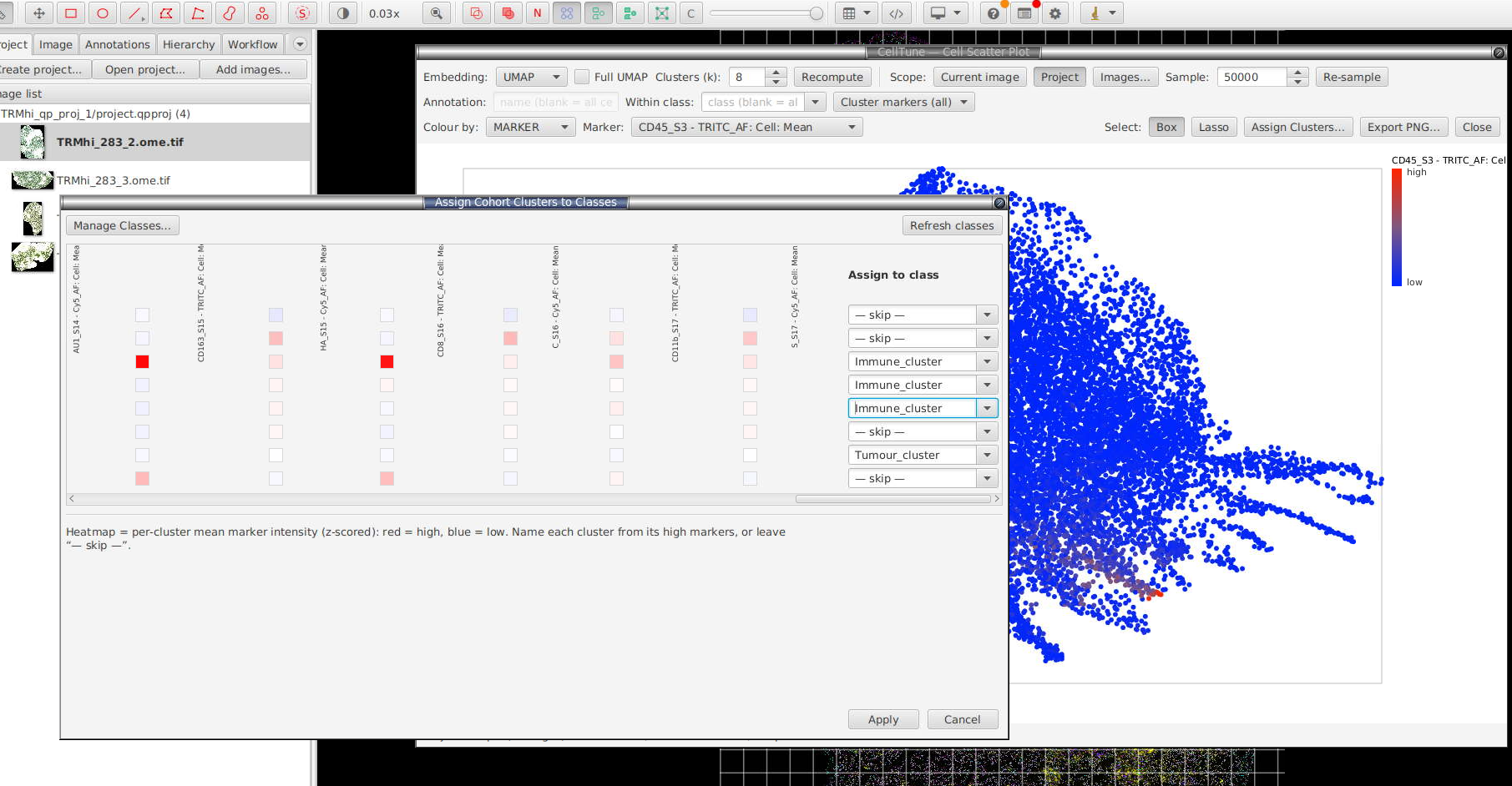
• Current-image scope (Apply Clusters…) — a second dialog shows the number of cells that will change. After you confirm, the chosen classes are written to those cells. Skipped clusters are not changed. Only the loaded cells are classified (at most the Sample: cap). To classify every cell in a large image, set Sample: to at least the image's cell count and click Re-sample, then Recompute, before applying.
• Project scope (Assign Clusters…) — see §11.5.

In both scopes, the new class replaces any existing class on the assigned cells. The extension's training labels are not changed.

11.4 Cluster-within-clusters (hierarchical gating)

Use the filter row to cluster inside one population (two-level phenotyping):

1. Cluster all cells on all markers → Apply Clusters… → assign the main classes (e.g. Tumour / Immune / Other).
2. Set Within class: Immune, open Cluster markers and tick only the immune markers (CD45, CD3d, CD8A, CD4, CD20, PD1, FOXP3) → Recompute. Only immune cells are clustered, on immune markers, z-scored within the immune cells.
3. Click Apply Clusters… again to name the subpopulations. Type names in the form Immune: CD8 T (QuPath treats Parent: Child as a derived class).

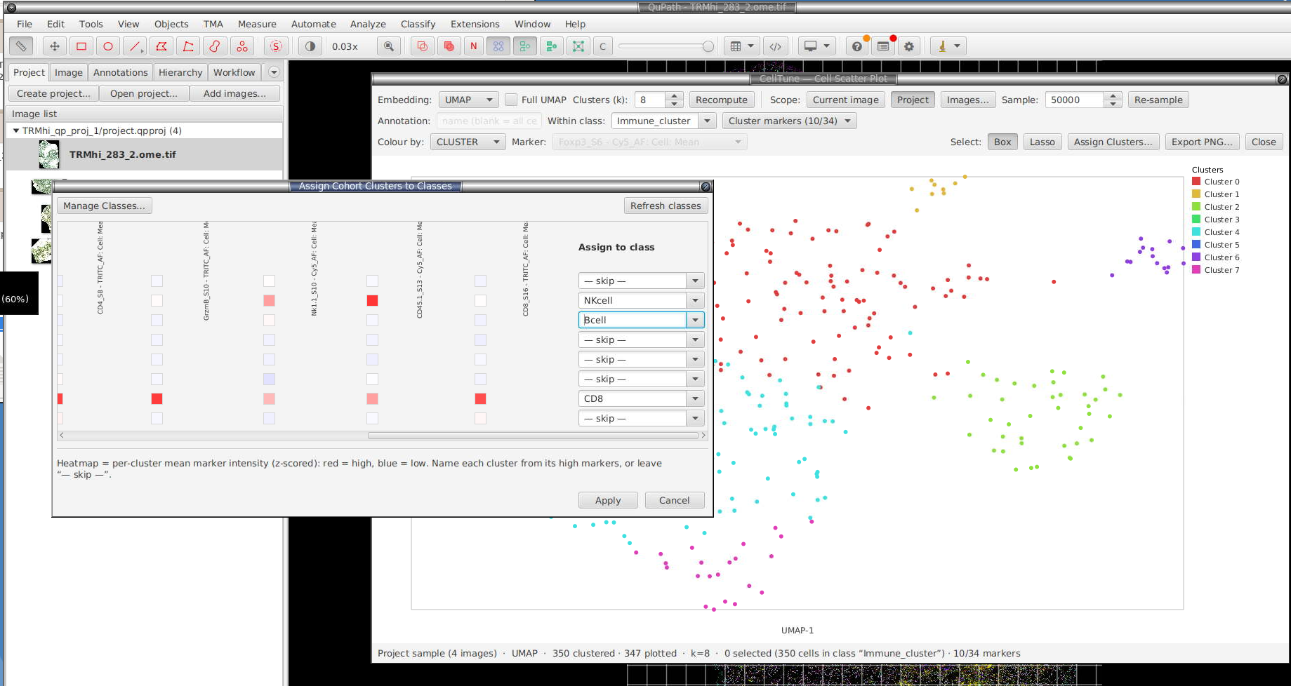
Repeat for further levels. The status bar shows the active filter and marker count, e.g. "(12,840 cells in class “Immune”) · 7/24 markers".

11.5 Project-wide clustering across images

Project scope fits one clustering on a sample of cells pooled from the images you choose, then applies it to every cell in those images. Cluster 3 then means the same population in every image. (If you cluster each image separately, the cluster numbers cannot be compared between images.) All controls in §11.1 work in project scope. Selection on the plot only highlights points (§11.2).

Entering project scope

1. Click Project. Choose the images to sample (all are selected by default). Click Cancel to stay on the current image.
2. Click Re-sample. The extension reads each image and takes up to Sample: ÷ (number of images) random cells from each, up to 50,000 in total by default. The status bar shows "Sampled X cell(s) across N image(s)".
3. Click Recompute to cluster the sample and draw the plot. (Clicking Recompute straight after step 1 does steps 2 and 3 together.)

The sample is only used to fit the clusters. When you assign, every cell in every selected image is assigned, one image at a time, so the number of images does not limit memory use. Raising Sample: above 50,000 makes the fit slower.

Working with the cohort sample

• Colour by → MARKER shows which clusters are high in which marker.
• Within class sub-clusters one population across all images. Assign Clusters… then changes only cells of that class.
• Cluster markers fits on a smaller panel.
• Recompute clusters the current sample again. To use different images, click Images… and then Re-sample. To change the sample size, change Sample: and click Re-sample. Then click Recompute.

Assigning across the cohort

Click Assign Clusters…. The dialog from §11.3 opens. After you confirm, each selected image is opened in turn, every matching cell is given its cluster's class, and the image is saved. Progress is shown in the status bar. (For how cells outside the sample are assigned, see §11.6.)

This changes every selected image. Assigning replaces the class on the assigned cells and saves each image. Training labels are not changed. The open image updates immediately.

Annotation filter. In project scope the Annotation filter limits which cells are sampled. With k-means, or Leiden Transfer from sample, Assign Clusters… and By cluster (all images) assign every cell in each image that passes Within class, including cells outside the matching annotations.

Staining differences between images. Normalisation is applied per marker, not per image. If one slide is stained brighter than the others, its cells can fall into different clusters. Check the per-image intensity distributions before pooling, and use batch normalisation (§19) with Use batch-corrected values ticked to correct them. The scatter plot then uses the corrected values in every scope and for every assign and write.

Leiden in project scope: Cluster all cells / Transfer from sample

With Method = Leiden and Scope = Project, two options appear next to Method:

• Cluster all cells (default) — clusters every cell in every selected image together, not just the sample. This is slower and uses more memory.
• Transfer from sample — clusters only the sample. Each other cell takes the most common cluster among its 15 nearest cells in the sample. This is faster.

With Cluster all cells, the full run is started by By cluster (all images):

1. Click Recompute to preview the clusters on the sample.
2. Click By cluster (all images) and confirm. The extension:
3. counts the cells first. If there are more than 50,000,000, it asks you to confirm again;
4. shows each step in the status bar: Pooling 12/40 images → Building kNN graph… → Running Leiden… → Writing 12/40 images;
5. writes a Cluster measurement to every cell and saves each image. Classifications are not changed;
6. shows a Cancel button. Cancelling stops before the next image. Images already written keep their new Cluster values.

When it finishes, the legend, the image colouring and the Assign Clusters… dialog show the clusters found across all cells. The plot itself still shows the sample. 3. Click Assign Clusters… to name the clusters. Classes are assigned from the written Cluster values.

If you click Assign Clusters… without step 2, or after a new Recompute, cells are assigned by transfer from the sample instead.

If the neighbour search is not accurate enough (below 95% recall), the run stops and an error dialog says that no Cluster measurement was written. Existing Cluster values are kept. Try different markers or more cells. The same check runs for Leiden on a single image or a project sample: if the status bar shows "Leiden preview: ANN recall too low — try more cells / different markers.", no clusters were made. Increase Sample: or change the ticked Cluster markers and click Recompute.

Comparison with scanpy. Results are similar to sc.tl.leiden in Python but not identical. This extension uses a different quality function (CPM rather than modularity) and weights the neighbour graph by shared neighbours (Jaccard) rather than UMAP connectivities. The same Resolution value can give slightly different cluster boundaries in scanpy.

Citing. If graph-based clustering is central to your analysis, cite the Leiden algorithm (Traag, Waltman & van Eck, Sci. Rep. 2019), scanpy (Wolf, Angerer & Theis, Genome Biol. 2018), whose scale → PCA → neighbours → Leiden steps this follows, and HNSW (Malkov & Yashunin, IEEE TPAMI 2020), used for the neighbour graph. Full citations and the licences of the bundled libraries (CWTS networkanalysis, jelmerk hnswlib-core) are in the README acknowledgements.

11.6 Clustering method: k-means vs Leiden

Method (§11.1) selects the clustering algorithm. All other controls work the same for both methods.

• k-means (default) splits cells into exactly k clusters (Clusters (k), 2–50, default 8). It works best when populations are of similar size.
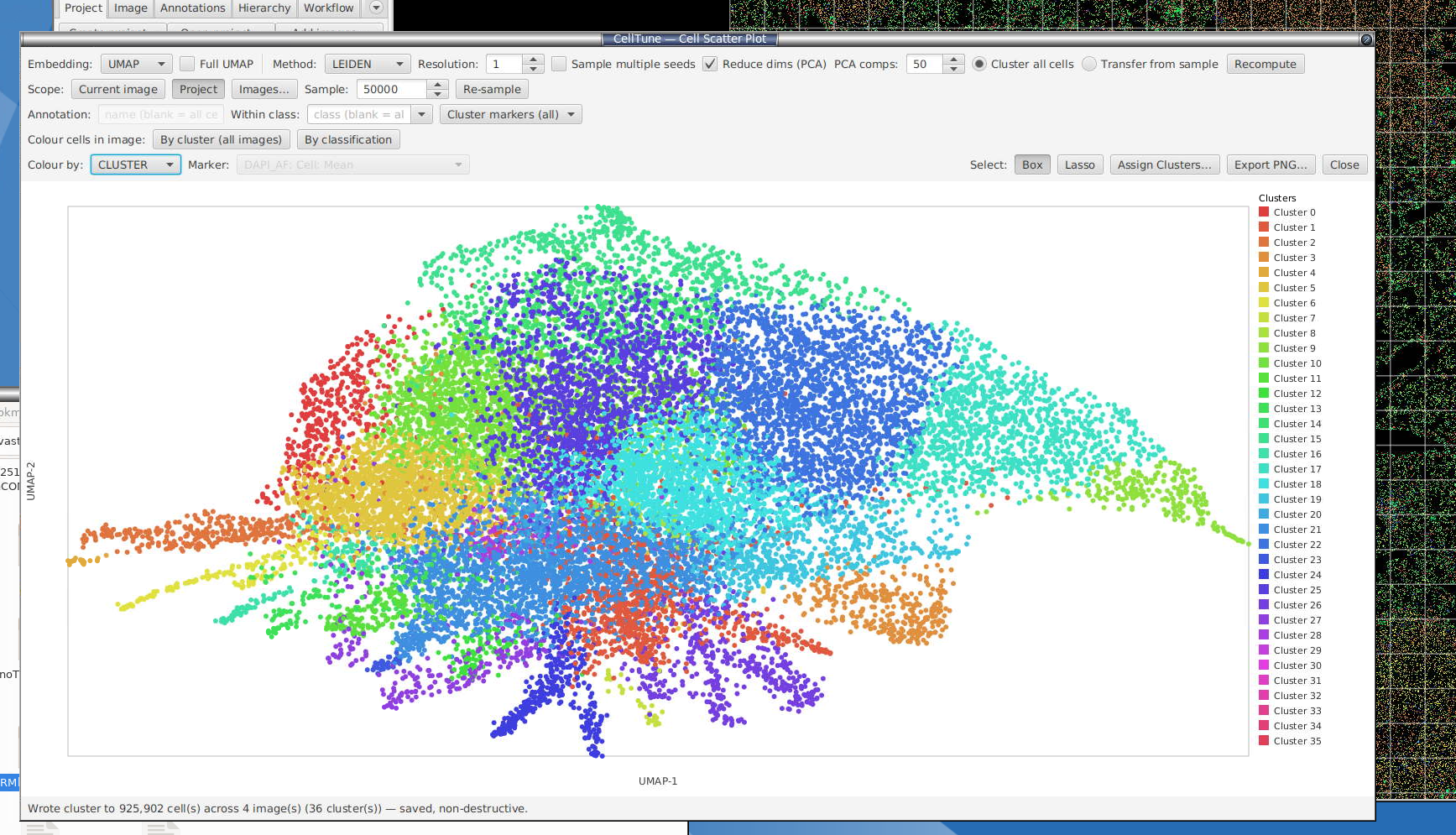
• Leiden links each cell to its 15 nearest cells (by marker values) and finds groups of closely linked cells. You set Resolution instead of a cluster count, and the number of clusters comes from the data. It is better than k-means at keeping small or unevenly sized populations as separate clusters. This is the method used by scanpy, scimap and SPACEc.

Controls when Method = Leiden

• Resolution (0.1–3.0, default 1.0) — replaces Clusters (k). Higher values give more, smaller clusters; lower values give fewer, larger clusters. After Recompute the status bar shows the number of clusters found, e.g. "7 cluster(s)". To get more or fewer clusters, raise or lower the resolution and click Recompute again.
• Sample multiple seeds — see §11.1. When ticked, Leiden runs 10 times with a fixed seed (42) and keeps the best result. When unticked, cluster numbers, and sometimes boundaries, can change between runs.

The neighbour count (15) and the edge weighting (shared-neighbour Jaccard) are fixed and cannot be changed in this version.

How cells outside the sample are assigned (project scope)

• k-means: each cell joins the cluster with the closest mean.
• Leiden, Transfer from sample: each cell takes the most common cluster among its 15 nearest cells in the sample.
• Leiden, Cluster all cells: all cells are clustered together, so no assignment step is needed (§11.5).

---