Project Prediction Summary¶
Experimental.
Menu: Extensions → SP Classify → Project Prediction Summary...
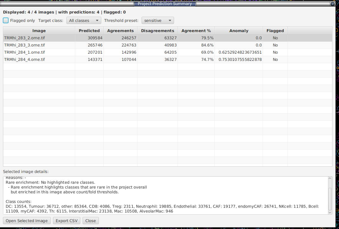
Shows one row per project image, using the saved predictions in <project>/celltune/image-predictions/, and gives each image an anomaly score so you can find the images to check first. See How the anomaly score is calculated. In binary mode it reads <project>/celltune/binary-image-predictions/<marker>/. An image whose saved predictions were made with a different class list shows Predictions made with a different class list. Apply the classifier to this image again. and gets no anomaly score.
To check images before cell segmentation, using pixel values only, see §17 Image pixel prescreen.
Table columns: Image, Predicted, Agreements, Disagreements, Agreement %, Anomaly, Flagged.
Filters:
- Flagged only: hide images that have no flag.
- Target class: show only images where the chosen class has the RARE_ENRICHMENT flag. The list contains only classes that have this flag in at least one image. Default: All classes.
- Threshold preset: hide unflagged images whose anomaly score is below the preset: strict 1.5, balanced 0.5, sensitive 0.0 (default; shows every image). Flagged images are always shown. The analysis is not re-run.
Buttons: - Open Selected Image: opens the selected image. - Export CSV: saves the rows currently shown as a CSV file.
⚠️ Open Selected Image discards unsaved changes in the current image without asking. Save first (File → Save) if you have made changes.
Details pane (below the table): for the selected image, shows the anomaly score, flag reasons, rare-class enrichment and the number of cells per class.
Anatomy of the anomaly score¶
For each image:
- Composition distance: how different the image's class proportions are from the whole project (Jensen-Shannon distance).
- Disagreement rate: disagreements ÷ predicted cells.
- Both values are converted to robust z-scores across all images. These use the median and the median absolute deviation (MAD), so one extreme image does not change the scale for the others.
Anomaly score = 0.65 × max(0, z_composition) + 0.35 × max(0, z_disagreement). Negative z-scores count as 0.
Composition has the larger weight because the disagreement rate partly depends on which two model types you chose. Use the score to rank images. It is not a probability.
Flag reasons:
- RARE_ENRICHMENT: a class that is under 1% of all cells in the project has at least 20 cells in this image and is at least 3× more common here than in the whole project.
- COMPOSITION_OUTLIER: composition z-score ≥ 3.
- HIGH_DISAGREEMENT: disagreement z-score ≥ 3.
How to use it: - Sort by Anomaly (the default sort). Check the top rows first. - Flagged with high disagreement: the classifier performs poorly on this image. Open it, label 10–20 cells, and retrain. - Composition outlier with low disagreement: either a real biological difference, or a staining or segmentation problem. Check the image visually. - Rare enrichment: check whether the cells really are that class, or are a staining or segmentation artefact.
With fewer than 5 images, the z-scores are unreliable.