Cellular neighborhoods (spatial micro-environments)

Menu: Extensions → SP Classify → Cellular Neighborhoods...

Cellular neighborhoods (CNs) group cells by the cell types around them, not by their own type. Each cell is described by the mix of cell types in its local window. These mixes are clustered into recurring micro-environments, such as tumour core, tumour–stroma interface or immune niches. This is the method of Schürch et al., "Coordinated Cellular Neighborhoods Orchestrate Antitumoral Immunity at the Colorectal Cancer Invasive Front," Cell 2020 (full citation & acknowledgement in the README). If you use this feature, please cite that paper.

Use this when cells of the same type behave differently depending on where they are, for example CD8 T cells inside tumour compared with CD8 T cells at the invasive margin. Instead of drawing tumour, stroma and interface regions by hand, k-means finds recurring neighbourhood compositions and labels every cell with one. You get a map in the viewer and a CN value on every cell, from which you can calculate the fraction of each image in each CN and compare across the cohort.

Results are written as new measurements (see §18.5). Cell classifications are not changed. You need cells that already have classifications, either from running the classifier or from an import.

18.1 When to use it

• You want to find tissue architecture (tumour, stroma, interface) or immune micro-environments (an activated-CD8 niche, a Treg-rich area) that a per-cell phenotype does not show.
• You want a per-image value that you can compare across a cohort, for example "the fraction of each patient's tissue in the activated-CD8 niche", for group comparisons.

18.2 How the clusters are computed

The same four steps run for one image or the whole project:

1. Neighbour window: for every cell, find the cells around it, using one of three modes. A cell is never counted as its own neighbour; Include centre cell in its own window adds it back (step 2).
2. k nearest neighbours: the window is a fixed number of cells (window (cells), default 10, range 2–100). With Include centre cell in its own window ticked, a window of 10 is the cell itself plus its 9 nearest neighbours, as in Schürch et al. With it unticked, it is the 10 nearest neighbours.
3. within radius: every cell within a set distance (default 50, range 5–500; µm if the image is calibrated, otherwise pixels).

4. Delaunay triangulation: neighbours are the cells directly connected to it in a triangulation, so the window size follows local cell density. Long connections across empty space are removed. Choose max edge for a fixed limit (default 50, range 1–2000; µm if calibrated, otherwise pixels) or auto (Q3+1.5·IQR) to set the limit separately for each image from its own connection lengths. A cell with no remaining connections gets CN = -1.

5. Composition vector: each window becomes a list of cell-type fractions (the proportion of Tumour, CD4 T, Treg, … in the window), using only the cell types you tick. With Include centre cell in its own window ticked (the default, as in the paper), the cell's own type is counted too. Cells of unticked types, unclassified cells and ignored classes are not counted. A window with no counted cells gets CN = -1 and is left out of clustering.

6. k-means clustering: the composition vectors are clustered into Number of CNs groups. Each group is one CN. Each cell's CN number (starting at 1) is written to the CN measurement; empty windows get -1. With Sample multiple k-means seeds (more reproducible) ticked (the default), k-means runs 10 times and keeps the best fit.

7. Interpretation: the mean composition of each CN is used for the enrichment heatmap and the diversity overlay.

Standardize compositions before clustering has the largest effect on results. Off (default, as in the paper): clusters separate the main tissue structure (tumour, stroma, interface). On: each cell type is scaled equally, so rare immune populations get their own clusters, but tumour and stroma merge into one or two large clusters. To get both, tick it, set Number of CNs to 12–15, and merge duplicate tumour clusters afterwards (§18.5).

A single k-means run depends on its random starting point. On test data, agreement with the published neighbourhoods varied a lot between starting points. Sample multiple k-means seeds (more reproducible) (on by default) runs k-means 10 times and keeps the best result, so repeated runs give the same answer. Untick it for a faster single run while you try out settings.

18.3 Scope: current image vs whole project

Scope, at the top of the dialog, sets what is clustered:

• Current image: clusters every non-empty window in the open image. Use it to try settings on one image.
• Whole project: fits one model across the images you choose, then writes a CN to every cell in every image. A CN number means the same micro-environment in every image (CN 3 is the same everywhere), so you can compare images. It runs in two passes and does not load the whole project into memory at once:
• Sample (fit): take a random sample of windows, drawn evenly from each selected image, and fit k-means on it. Sample windows for fit (default 50,000, range 1,000–5,000,000) sets how many windows are used. Every cell is still assigned afterwards.
• Assign: for each image, calculate every cell's composition, assign it to the nearest CN, write the CN measurement, and save the image.

Selecting Whole project shows Choose images…, Add project…, Sample windows for fit and Parallel workers (§18.6).

Clustering more than one project together

To fit one model across several QuPath projects (for example two staining batches), click Add project… (next to Also cluster projects:) and select the other project's project.qpproj. All images in each added project are included, together with the images you selected in this project. Each image's results are saved in its own project. No files are copied between projects. Clear removes the added projects.

Projects clustered together must use the same cell class names, because compositions are matched by class name. Separately stained cohorts can also differ by batch: compare per-project CN fractions, and consider Standardize compositions before clustering (§18.2). The cell-type list comes from the open image, so open a typical image before you run.

18.4 Running it — step by step

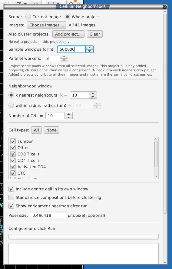
The dialog set up for a whole-project run. The current version has an extra option, Sample multiple k-means seeds (more reproducible), and the kNN control is labelled window (cells).

1. Open Extensions → SP Classify → Cellular Neighborhoods.... Choose Scope. For Whole project, click Choose images…, and Add project… to include other projects.
2. Choose the Neighborhood window (see §18.2). Use within radius for a fixed physical distance on calibrated images, or Delaunay triangulation when cell density varies a lot.
3. Set Number of CNs (default 10, range 2–30). Fewer gives broader regions. More gives finer regions, some of which you may need to merge.
4. Tick the Cell types to include (All / None tick or untick every type). Leave out debris and ignored classes.
5. Set the options: Include centre cell in its own window (leave ticked to match the paper), Standardize compositions before clustering (§18.2), Sample multiple k-means seeds (more reproducible) (leave ticked), Show enrichment heatmap after run.
6. Pixel size (µm/pixel, optional) is filled in from the image calibration. For uncalibrated images, set it if you want the radius in µm.
7. For project scope, check Sample windows for fit (default 50,000) and Parallel workers (default: number of CPU cores minus 1, up to 8; see §18.6).
8. Click Run. The log shows progress. In project scope, each image logs a sampled … line and then a CN assigned … line; lines from different workers are mixed together.

18.5 The enrichment heatmap — reading, naming, merging

The CN-by-cell-type enrichment heatmap opens after a run if Show enrichment heatmap after run is ticked, or when you click Show heatmap:

• Rows = CNs, with cell counts and % of all cells. Columns = cell types.
• Numbers = each CN's mean fraction of each cell type (shown when Show mean fractions is ticked).
• Colour = z-score of each cell type across the CNs. Red means more of that cell type than in the other CNs, and blue means less, so a cell type that is low in absolute terms but higher than in other CNs is still shown in red. Read the colour (which type defines the CN) together with the number (how much of it there is).

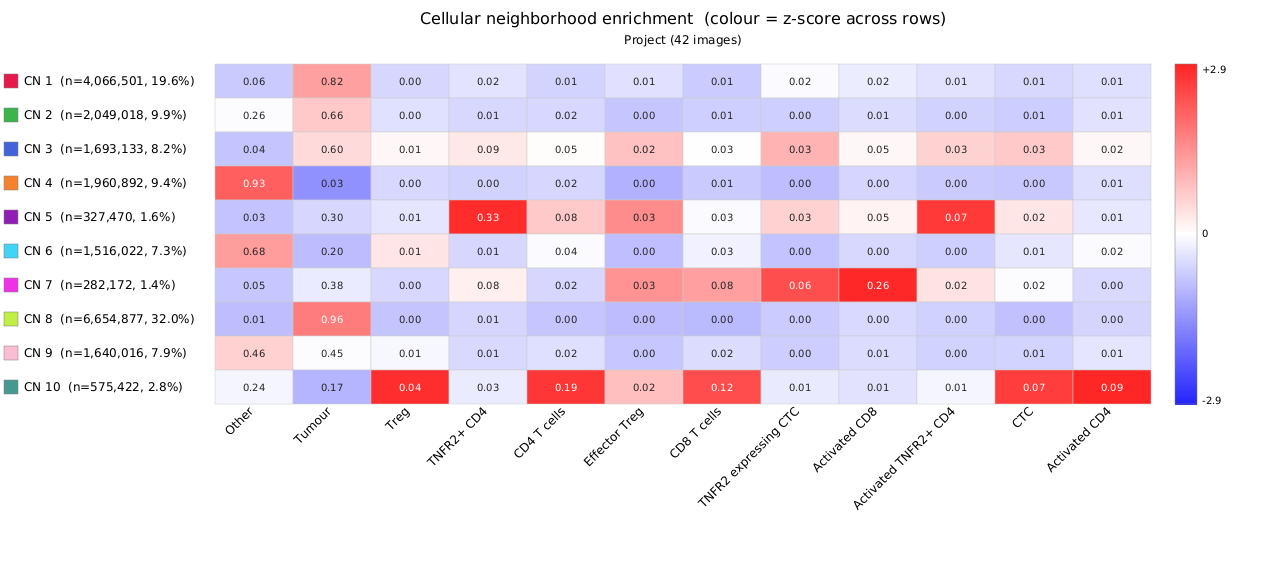
A 10-CN result for a whole project. CN 8 and CN 1 are mostly tumour (32% and 20% of cells). CN 4 is stroma/other. CN 5, 7 and 10 are small immune-rich neighbourhoods (1–3% of cells). CNs 1, 2, 8 and 9 are all tumour-dominated; give them the same name to merge them (below).

Name / merge: type a name next to each CN and click Apply names. Results appear as columns in the detection measurement table and in cell-table exports (§12.1). None of them change cell classifications.

Result	Written when	Stored as	Key	Values
Raw cluster id	Run	numeric measurement	CN	1..k (empty-window cells = -1)
Named class (readable)	Apply names	text metadata string	CN Class	the name you typed (empty-window cells = Unassigned)
Named class (numeric)	Apply names	numeric measurement	CN Class code	1..m (used by the Color by: CN Class overlay)

Giving two CNs the same name merges them. Only CN Class and CN Class code change; CN keeps the original cluster numbers. CN Class is stored as text in the cell's metadata, so in Export → Cell Table... you must tick it in the column list. It is listed after the numeric measurements.

Saving. In project scope, Apply names updates and saves every image from the run, using the Parallel workers count. The open image is updated and saved too. In current-image scope it updates only the open image and does not save it; press Ctrl+S to save.

Export: Export as PNG… saves the heatmap. Export CN frequencies CSV… saves one row per CN: cell count, fraction of all cells, diversity, and the mean fraction of each cell type. For CN fractions per image, export the cell table (§12.1) with the CN or CN Class column and count the cells in each image. Use these to check whether CN frequencies follow your biological groups or your staining batches.

18.6 Parallel workers (project scope) — performance

Parallel workers (default: number of CPU cores minus 1, up to 8) sets how many images are processed at once, in both the sample and the assign pass. Each worker loads one whole image's cells, so memory use rises with the worker count.

• For images with hundreds of thousands of cells, use 2–4 workers.
• For many small images, use more workers.
• Results are the same for any worker count.

18.7 Viewer overlays

Three buttons recolour the viewer using the last run. They do not change the cells. Cells with CN = -1 keep their classification colour.

• Color by: Neighborhood (CN): one colour per CN. CNs that touch in the tissue get contrasting colours.
• Color by: CN Class: one colour per named class, after Apply names (uses CN Class code).
• Color by: diversity: colours each cell by the Shannon diversity of the cell types in its window (0 = one cell type, 1 = an even mix). Use it to find mixed zones and interfaces.

Click a button again to return to classification colours. Closing the dialog also returns the viewer to classification colours.

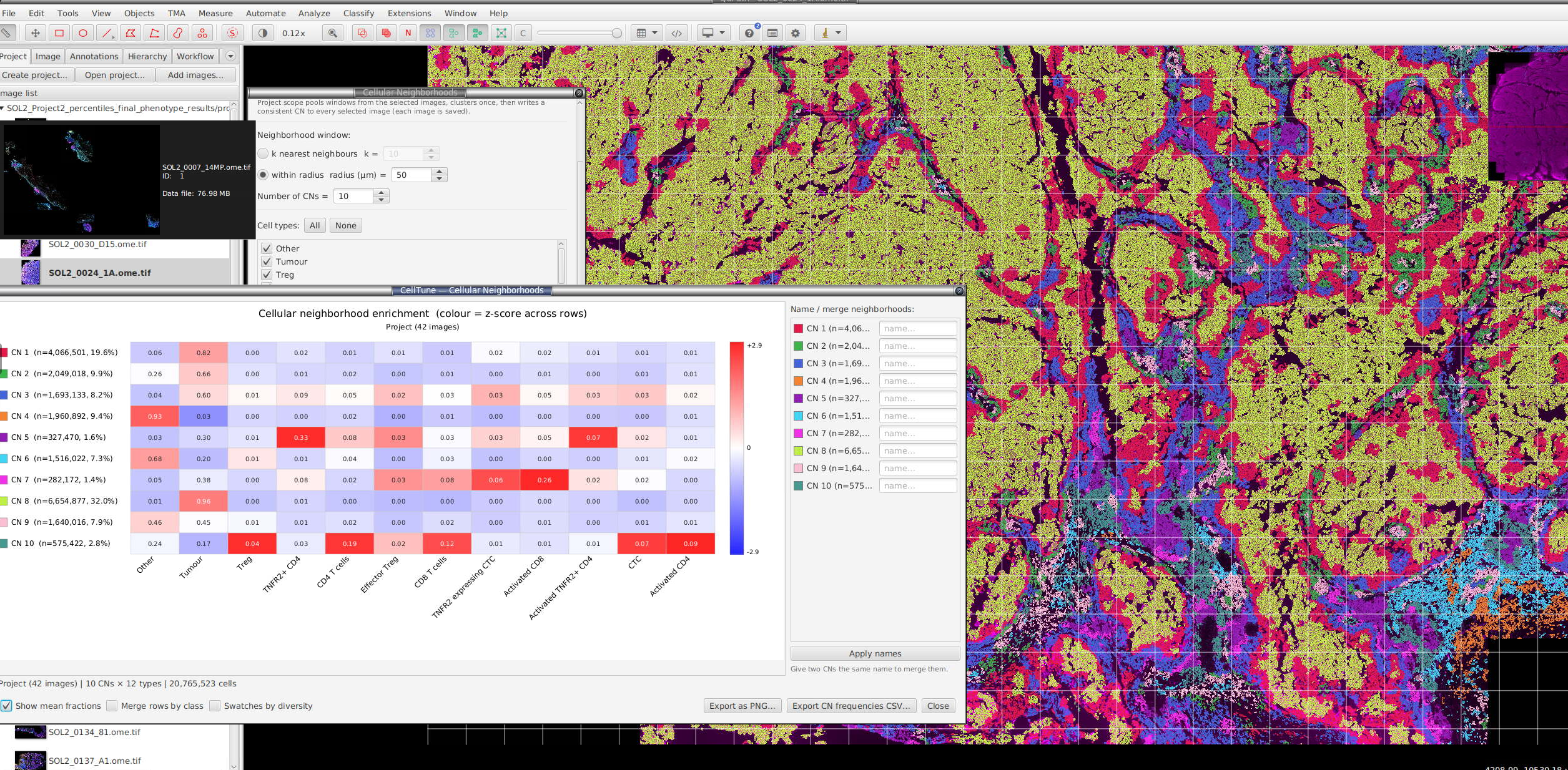
The Color by: Neighborhood (CN) overlay, with the enrichment heatmap and the Name / merge neighborhoods panel. Neighbouring CNs get contrasting colours.

18.8 Tips & cautions

• Check that differences in CN frequency are biological. Differences between samples are usually the result you are looking for. But CNs are built from your cell classifications, so any staining or batch effect in classification carries into the CN frequencies. Compare per-image CN fractions between your groups and between your batches.
• Check CNs that come mostly from one or two images. Such a CN may reflect one unusual slide rather than shared biology. CNs with less than 2% of cells are the least stable; confirm that they appear again (for example in another cohort or a repeat run) before you interpret them.
• Run the classifier first. CN results depend on the quality of the cell classifications.
• within radius vs k nearest neighbours: with within radius, dense regions have more cells per window. With k nearest neighbours, every window has the same number of cells, so density does not change window size. Choose the mode that suits your question.

---